YES function: Manage it perfectly in 4 steps

​The function YEAH Excel is one of the most used functions since it tests whether a condition is met or not. In this article you will quickly learn how to use it.

Key information:

This function allows you to evaluate a condition. Excel checks if the logical test is met and delivers different results. The first result is delivered when the evaluation is true, the second if it is false.  

How does it work?

• Purpose: The IF function allows us to evaluate whether a condition is true or false. If true, it performs a given action, otherwise it performs another action. 
• Characteristics:It allows you to evaluate with different symbols, for example, equal, less, greater than or equal, unequal, etc. Numeric or text values can also be evaluated in the logic test.
• Syntax:​​​​​​ =IF(logical_test; [value_if_true]; [value_if_false]
• Arguments:
  • logical_test: Value or expression that we seek to evaluate.
  • value_if_true: Value returned when the evaluation is true. This value can be text, calculations, a reference to another cell, or other functions.
  • value_if_false: Value returned when the evaluation is false. This argument is optional, if not set, Excel will respond “FALSE” automatically.

Step 1: Understanding the IF function

The Excel IF function is used in different situations. It allows you to verify logical tests by delivering different values if it is true or false. To understand better, let's look at the diagram,

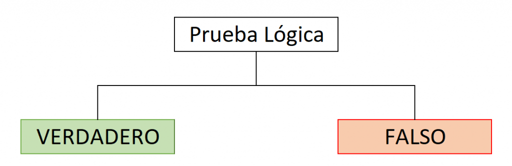
Excel will check the condition, delivering a different result in each case. Logical tests and results can be numerical values, texts, mathematical operations, or formulas.

We recommend the following video to understand how SI works.

Step 2: Using the IF function

Evaluating numerical conditions

The formula allows you to verify numerical tests. When we have text arguments we must write it in quotes. For example, the formula can be used to categorize people into majors and minors.

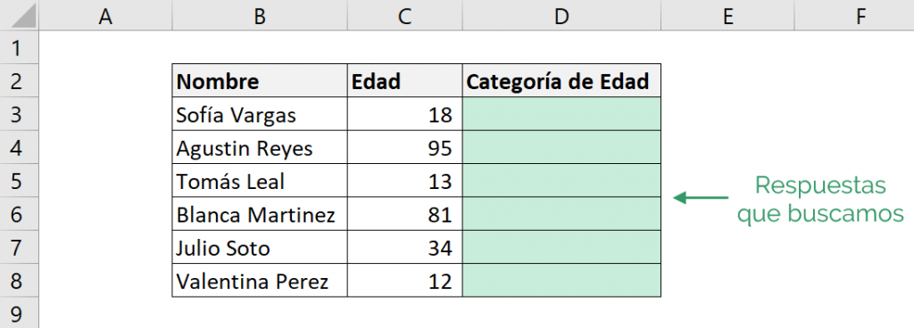
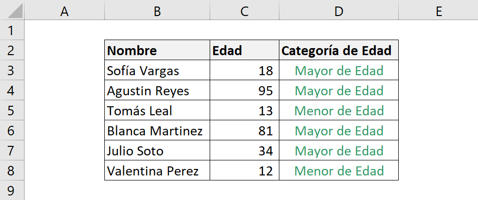
Excel evaluates whether you are of legal age by providing a response “Of Legal Age”, if your age is greater than or equal to 18 years, and “Minor”, if your age is less. 

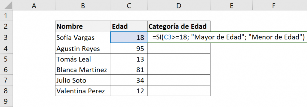
The elements of the function are:

• logic_test:  C3>=18
• value_if_true: “Adult"
• value_if_false:  "Younger"

That is, the IF function is:

What it means is: “If Sofia's age is greater than or equal to 18, the IF function responds Adult, otherwise, respond Younger”

The result we will obtain will be:

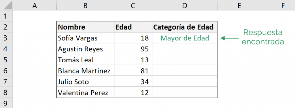
We can verify that Sofia's age is 18 years old, and since it is equal to 18, it is adult, agreeing with the answer.

We do this for all people:

Evaluating text conditions

The IF function also evaluates text logistic tests. Continuing with the example, we want the adult category to get a discount. 

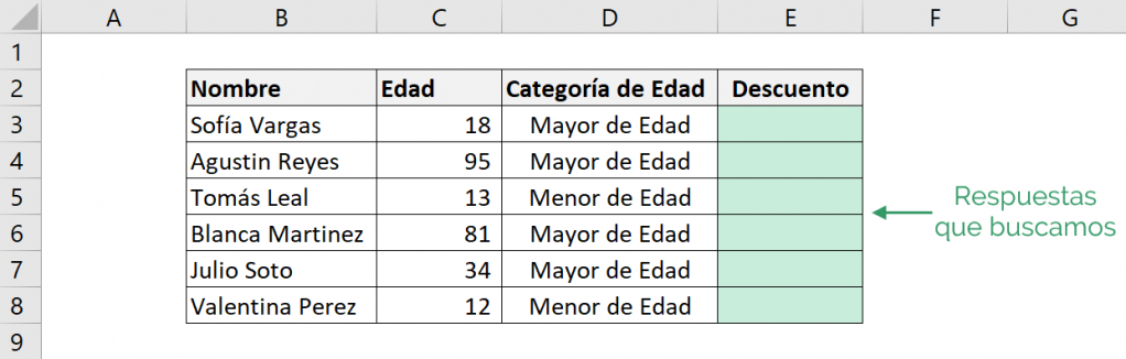
Excel evaluates the age category, responding Yeah, if you are of legal age or responding No, if it doesn't match.  

Therefore, the elements that the function will have are:

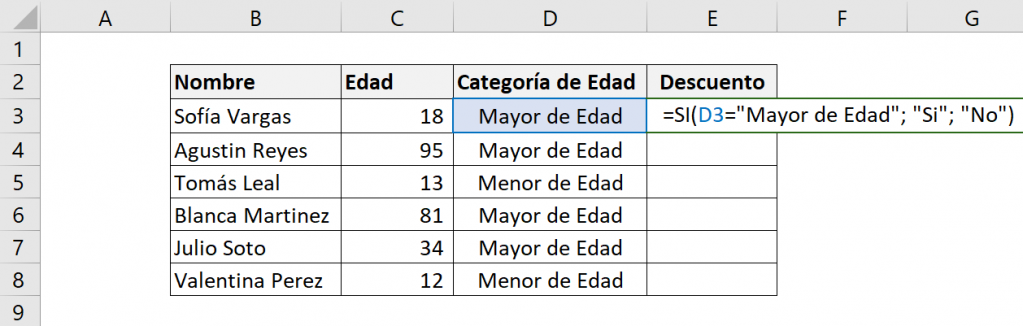
• logic_test:  D3=”Of Age”
• value_if_true:  Yeah
• value_if_false:  No

That is, the IF function is:

What it means is: “If Sofia's age category is Adult, the IF function responds Yeah, otherwise, respond No”

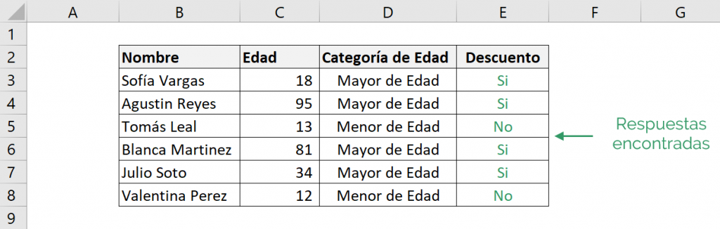
The result we will obtain will be:

Step 3: Combine the IF function with the OR and AND functions

By using the IF function in conjunction with the OR and AND formulas you will become a true Excel Ninja. 

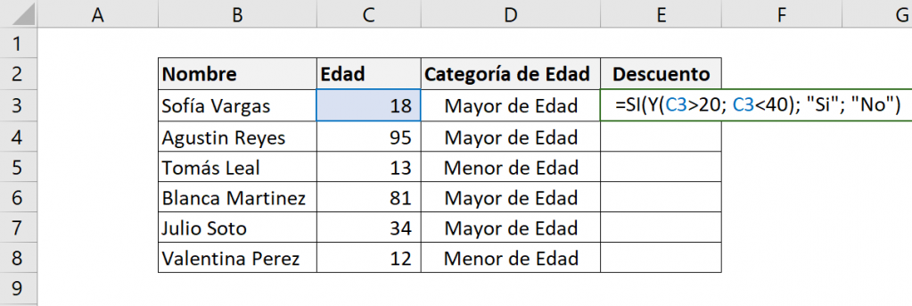
To combine them correctly, we must include these functions in the logical test of the IF formula. Continuing with the example, if a person's age is between 20 and 40 years old, they will be given a discount. We use the AND function.

Therefore, the elements that the function will have are:

• logic_test:  Y(C3>20; C3<40)
• value_if_true:  Yeah
• value_if_false:  No

That is, the IF function is:

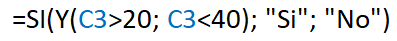
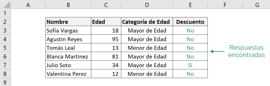
What it means is: “If Sofia's age is greater than 20 and less than 40 years old, the SI function responds Yeah, otherwise, respond No”

The result we will obtain will be:

Ninja Tip: Visit the following article to delve deeper into the combination of IF and AND functions.

Step 4: Nested IF Function

Nested IF function is used when we need to evaluate more than one logical test and get more than two answers. For this, we have to add an IF function, inside the main IF formula. The schematic shows how it works.

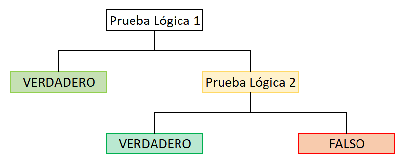
In the event that logical test 1 is satisfied, Excel responds TRUE. In the event that it is not met, Excel will evaluate the second logical test and depending on whether it is met, it returns TRUE or FALSE.  

In the example, we want to add the elderly category. We consider a senior citizen when their age is greater than or equal to 65 years.

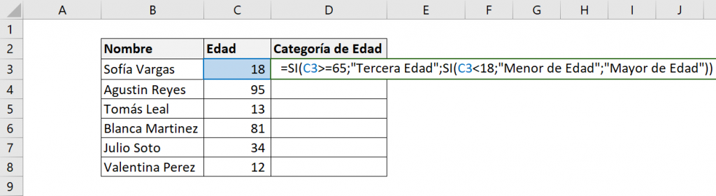
Therefore, the elements that the function will have are:

• logic_test:  C3>=65
• value_if_true:  “Third age”
• value_if_false:  IF function:
  • Logic test:  C3<18
  • value_if_true:  "Younger"
  • value_if_false:  "Adult"

That is, the IF function is:

What it means is: “If Sofia's age is greater than or equal to 65, the IF function responds Third Age, otherwise, the second logical test will be evaluated, which consists of: if Sofia's age is less than 18, answer Younger, otherwise, respond Adult”

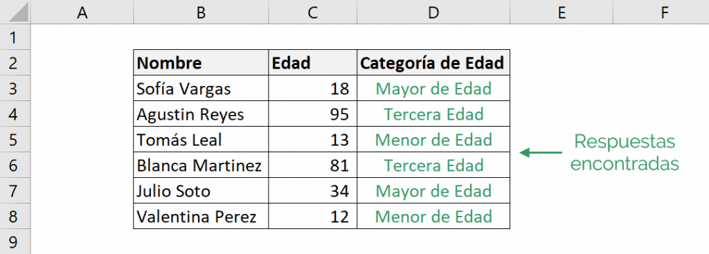
Ninja Tip: When we want to perform many logical tests, using the nested IF function can be very complicated, so we recommend using the IF.SET formula that allows you to perform up to 127 logical tests.

Common mistakes

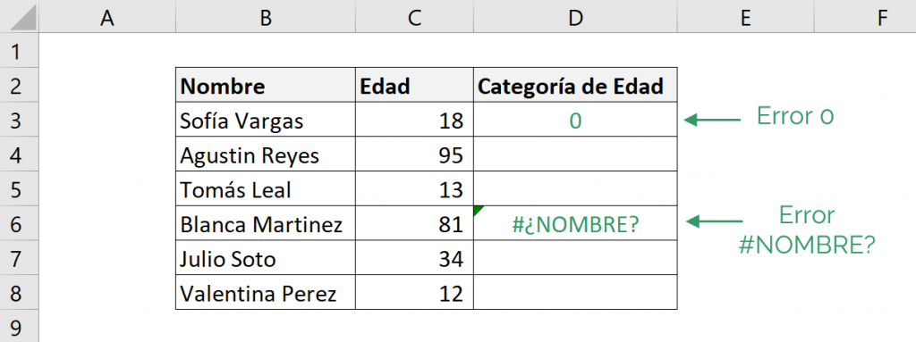
*IF function answers 0

On some occasions it may respond with a “0”. This error usually indicates that a value was not defined for the true and false arguments. 

If this happens to you, we recommend giving value to the true and false arguments.

* #NAME?

This error usually indicates that there is an error in the formula. We advise you to review the following points:

• Check that the text values for true and false are in quotes.
• Make sure the logical proof is set up correctly.

Ninja Tip:  You can use the IF.ERROR or IF.ND functions to handle errors.  

Frequent questions